A convnet takes as input of shape (image_height, image_width, image_channels). Here, our input images are of shape (28,28,1) so we specify input_shape = c(28,28,1).
The 1st layer is specialised to perform the convolution operation. We’ll see what this means later. It has 32 hidden units, a kernel size of 3x3, ReLU Activation.
The 1st layer is followed by a Max Pooling Layer with pool size of 2x2.
The next Convolution layer has 64 hidden units followed by a Max pooling layer.
Now, the output of every Convolution and Max Pooling Layer is a 3d tensor of shape (height, width, channels). So, we feed an image and get something we call a Feature Map.
This Feature Map represent, as the name suggests, various features present in the image we input. Imagine the Feature Map as a matrix with numbers which indicate the presence of a feature. If the number is big, the feature is more likely to be there. The Max Pooling layer looks at the feature map, and extracts a smaller map where only the big numbers are present (i.e. max values are there thus, max pooling).
So, as we move deeper into the network, this maps keeps shrinking in size. We start with an image of size (28,28) with 1 channel and end up with a feature map which is a 3x3 matrix with 64 channels.
This feature map has to be re-shaped so that we can feed it into a dense neural network. For this we use a Flatten Layer which compressed the 3d map of shape (3,3,64) into a 1d vector of size 576.
Then we have a densely connected layer with 64 hidden units which is then connected to a 10-hidden units layer with softmax activation. This last layer gives us the probabilities for different Digits.
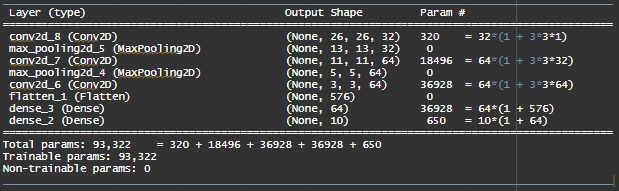
Model Structure
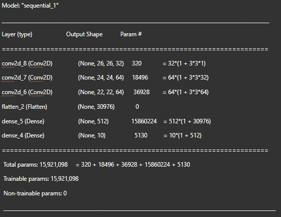
We can calculate the number of parameters of layers using this generalisation : (1 + width* height* No. of filters_previous layer)* No. of filters_current layer.
So, the Parameters in the 2nd Convolution Layer = 18496 = 64*(1 + 3 * 3 * 32)
We add ‘1’ because we have 1 Bias Term.
The Pooling Layers don’t have any parameters because all it does is takes the maximum of numbers of the previous layer. Thus, there is no learning involved here.
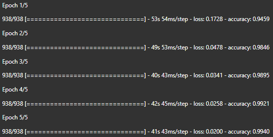
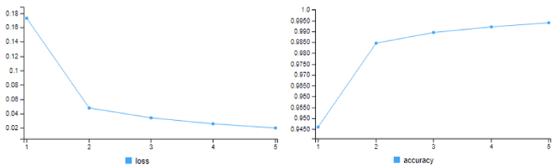
We end up with a training accuracy of 99.40% and test accuracy of 99.26%
Model
Training Accuracy
Test Accuracy
Dense Neural Network
98.86 %
98.15 %
Convolution Neural Network
99.40 %
99.26 %
The Dense Neural Network has a very high accuracy for both the Training and Test Datasets. However the Convolution Neural Network easily outperformed the DNN !
Understanding What Happened
Dense layers -vs- Convolution layers
A Dense Layer learns the global features from the input feature space (for e.g. the digit patterns of our MNIST images). Whereas, a Convolution Layer learns the local patterns found in a small 2d window. We specify the window size using kernel_size = c(3 , 3) i.e. a 3x3 window.
These patterns learnt by the CNN are Translation Invariant and the convolution layers can learn spatial hierarchy of patterns.
Translation Invariant means that a local-pattern learnt somewhere can be identified elsewhere. This is not the case for densely connected network as they learn every pattern anew at every new location.
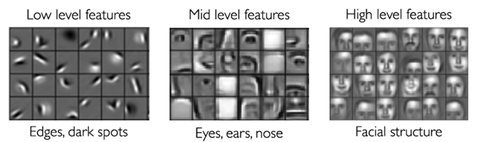
Spatial Hierarchy Learning means that the 1st layer picks up smaller local patterns like edges - 2nd layer picks up larger patterns made of features of the previous layer.
This 1st property makes convolution layers data efficient and have better generalisation capacity. The 2nd property makes convolution layers efficient in learning complex and abstract ideas.
Spatial Hierarchy of Representations
Our input for a CNN is a picture i.e. 3d tensor of shape (height, width, channel) where channel = 1 for black and white, while 3 for RGB i.e. colour image. This input picture is called a feature map <> height and width are called spatial axes <> channel is also depth axis.
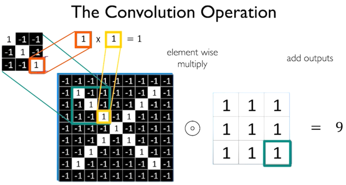
The Convolution Operation
The network extracts patches from its input feature map -> apply a transformation -> output feature map (also a 3d tensor). The output 3d tensor has shape (height, width, depth).
However, the output depth does not represent colour channels - rather it represents filters which encodes specific aspect about the input image. Here, depth/filters is a parameter we specific in our layer for e.g. above network for MNIST dataset.
Convolution Operation
The 1st layer has input feature map of (28,28,1) -> output map (26,26,32). Here, 32 is the number of filters we specified. Each of the 32 output channels contains 26 by 26 grid of values - we call this a “response/feaure map”.
The convolution operation works by sliding these windows of size 3x3 over the 3d input feature map, stopping at every possible location and extracting a 3d patch of surrounding features. Each such 3d patch is then transformed i.e. dot product with a weight matrix - which we call “convolution kernel”. 3d patch -> 1d vector of shape (output_depth). All such 1d vectors are spatially reassembled into a 3d output map of shape (height, width, output_depth) for eg. (26,26,32).
Every spatial location in the output feature map corresponds to the same location in the input feature map (for example, the lower-right corner of the output contains information about the lower-right corner of the input)
Now, we enter the max_pooling_layer - here the input is a 26x26 feature map which the max pooling layer halved into 13x13 - aggressive down-sampling. It extracts windows from the input feature maps and outputs the max value of every channel. Max Pooling is generally done using window 2x2 and stride 2 (thus, halves the input) whereas, a convolution involves 3x3 or 5x5 with stride = 1.
Border effect and Padding
Our input feature map is 28x28 which gets reduced to 26x26, why? Say, we have a 5x5 feature map and a 3x3 patch we drag along - there are only 9 tiles where we can centre this patch - as a result of which we end up with a shrunk output feature map. This is called border effect. Solution? Padding.
If we want the dimensions to be same, we need to add appropriate number of rows and columns on each side so that we can centre the patch accordingly.
for a 3x3 patch, we add 1 row and column on all sides
for a 5x5 patch, we add 2 rows and columns on all sides
How is it achieved? We mention padding = “valid” (i.e. no padding, default configuration) or “same” (yes to padding)
Strides
By how much does the patch need to move ? This is a parameter called “strides” which we can specify. The default value = 1. When we use stride = 2 we end up with an output feature map which is down-sampled by a factor of 2 - such a convolution is called Strided CNN. For down-sampling, we prefer “pooling” over “strides” because pooling can work more aggressively.
Need for Pooling ?
Figure : Max Pooling
Pooling primarily helps us reduce dimensionality making the model scalable while preserving the spatial invariance/structure. If we have a model without pooling, it looks like this :-
15 million! is a very high number of parameters given the size of our model. Thus, we can expected there to be intense overfitting.
This model is not good for learning spatial hierarchy of features because the 3x3 window in the later layers do not see the totality of the input image so it cannot learn high level features.
Ways of down-pooling : (1) using strides (2) pooling : max or average
Why Max pooling works better :
Features tend to encode the spatial presence of some pattern/concept over the different tiles of the feature map.
It’s more informative to look at the maximal presence of different features than at their average presence.
Strided convolution/average pooling could end up diluting or missing feature-presence information.
Let’s explore more about Convolution Neural Networks !